October 18, 2020
Alejandra Plazola and MAP5667
Data Wrangling and Data Exploration
Dog popularity, intelligence, and breed info.
Introduction
Recently, I have been into dogs and raising my pups, I did quite a bit of background research on dog breeds before selecting which breed was the best at fitting into my lifestyle plus my past experiences of raising certain dog breeds like German Shepherds, Labs, and Rottweilers.
This got me to thinking that I automatically wanted to do my project one over dog breed intelligence and comparing it to dog breed popularity.I wanted to compare dogs intelligence and see if intelligence is a type of trait that people are interested in when picking a dog and it's overall popularity for that breed.
I have chosen 3 data sets "AKC_Popularity_Breeds_2013-2019", "AKC Breed Info" and "dog_intelligence". These datasets were obtained through dataworld:https://data.world/len/akc-popular-dog-breeds, https://data.world/len/dog-canine-breed-size-akc, and https://data.world/len/intelligence-of-dogs. (For some reason data world doesn't connect through html here but it does if you open the link in a new tab.)
For the "dog_intelligence" dataset it contains 5 different variables, Breed = dog breed, Classification = what type of dog the breed is categorized, obey = the probability that the breed obeys the first command, reps_lower= lower limit of repetitions the breed takes to understand new commands, and reps_upper= upper limit of repetitions the breed takes to understand new commands. This dataset has 136 observations in total.
For the "AKC_Popular_Breeds_2013-2019" dataset, it has 8 variables and 193 observations. The 8 different variables are Breed= dog breed,and then popularity ranking for each year from 2013-2019 (Rank 2013, Rank 2014, Rank 2015, Rank 2016, Rank 2017, Rank 2018, and Rank 2019). I also updated this dataset from it's original on dataworld to include more recent rankings.
The new rankings sources I added from 2017-19 used was from: https://www.akc.org/expert-advice/news/most-popular-dog-breeds-full-ranking-list/ and https://www.akc.org/expert-advice/dog-breeds/2020-popular-breeds-2019/. There was a ranking from 2020, but it was a predicted one and since the year is not over I did not want to include it.
To reiterate these are interesting because I see that some people get certain dog breeds because their family or friends have them, sometimes they see it off a movie/tv show, or even know the type of dog they want such as a working breed, herding dog type, guard dogs, etc. I wanted to see if intelligence plays a big role in popularity of dogs as I know that most of the dogs I've had growing up were due to the stigma around the breed, such as they are smart or amazing guard dogs. Over the summer my family got two new puppies, a Beglian Malinois, and a Great Pyrenees/German Shepherd mix. They were picked because they are known to be good guard dogs/working dogs, considered very bright, and that was something my father wanted for the home, also they are good family companions. Another factor that people use to choose animals is their size, many people like bigger breeds and others like smaller.
I want to see if there is a correlation between popularity of dog breeds between it's intelligence rank, and it's size. I predict people will choose dog breeds that are the smartest.
Tidying and Joining/Merging
library(tidyverse)
Dogp <- read_csv("/stor/home/map5667/Website/content/project/AKC_Popular_Breeds_2013-2019.csv")
Dogint <- read_csv("/stor/home/map5667/Website/content/project/dog_intelligence.csv")
Dogbreed <- read_csv("/stor/home/map5667/Website/content/project/AKC Breed Info.csv")
# tidying only Dog popularity ranks
Dogpp <- Dogp %>% rename(`2019` = "2019 Rank", `2018` = "2018 Rank",
    `2017` = "2017 Rank", `2016` = "2016 Rank", `2015` = "2015 Rank",
    `2014` = "2014 Rank", `2013` = "2013 Rank")
Dogpop <- Dogpp %>% pivot_longer(cols = c("2013", "2014", "2015",
    "2016", "2017", "2018", "2019"), names_to = "Year", values_to = "Rank") %>%
    na.omit
Dogpop %>% glimpse()
## Rows: 1,309
## Columns: 3
## $ Breed <chr> "American Water Spaniel", "American Water Spaniel", "American W…
## $ Year <chr> "2013", "2014", "2015", "2016", "2017", "2018", "2019", "2013",…
## $ Rank <dbl> 144, 160, 157, 156, 167, 166, 164, 143, 144, 136, 149, 147, 148…Dogpop %>% summarize_all(n_distinct)## # A tibble: 1 x 3
## Breed Year Rank
## <int> <int> <int>
## 1 193 7 193I first renamed all year ranks and pivoted longer into a seperate column by year and rank for the dog popularity dataset and omitted any n/a rows from the set
Dogintel <- Dogint %>% rename(Lower = "reps_lower", Upper = "reps_upper") %>%
    pivot_longer(cols = c("Lower", "Upper"), names_to = "Reps",
        values_to = "Repnum")
Dogin <- Dogintel %>% group_by(Breed) %>% mutate(avgReps = mean(Repnum,
    na.rm = T)) %>% select(-Repnum, -Reps) %>% distinct()
Dogin %>% glimpse()
## Rows: 136
## Columns: 4
## Groups: Breed [136]
## $ Breed <chr> "Affenpinscher", "Afghan Hound", "Airedale Terrier", "…
## $ Classification <chr> "Above Average Working Dogs", "Lowest Degree of Workin…
## $ obey <chr> "70%", NA, "70%", "50%", "50%", "50%", "70%", "50%", "…
## $ avgReps <dbl> 20.5, 90.5, 20.5, 33.0, 33.0, 33.0, 20.5, 33.0, 2.5, 3…Dogin %>% head()## # A tibble: 6 x 4
## # Groups: Breed [6]
## Breed Classification obey avgReps
## <chr> <chr> <chr> <dbl>
## 1 Affenpinscher Above Average Working Dogs 70% 20.5
## 2 Afghan Hound Lowest Degree of Working/Obedience Intelligen… <NA> 90.5
## 3 Airedale Terrier Above Average Working Dogs 70% 20.5
## 4 Akita Average Working/Obedience Intelligence 50% 33
## 5 Alaskan Malamute Average Working/Obedience Intelligence 50% 33
## 6 American Foxhound Average Working/Obedience Intelligence 50% 33Dogbd <- Dogbreed %>% rename(Low.ht = "height_low_inches", High.ht = "height_high_inches",
Low.wt = "weight_low_lbs", High.wt = "weight_high_lbs") %>%
pivot_longer(cols = c("Low.ht", "High.ht"), names_to = "Ht",
values_to = "Ht.inch") %>% pivot_longer(cols = c("Low.wt",
"High.wt"), names_to = "Wt", values_to = "Wt.lbs")
Dogbdinfo <- Dogbd %>% na.omit() %>% group_by(Breed) %>% mutate(avght = mean(Ht.inch,
na.rm = T), avgwt = mean(Wt.lbs, na.rm = T)) %>% select(-Ht.inch,
-Ht, -Wt.lbs, -Wt) %>% distinct()
Dogbdinfo %>% glimpse()## Rows: 148
## Columns: 3
## Groups: Breed [148]
## $ Breed <chr> "Affenpinscher", "Afghan Hound", "Airdale Terrier", "Akita", "A…
## $ avght <dbl> 10.5, 26.0, 23.0, 27.0, 14.0, 23.5, 18.0, 16.5, 28.0, 18.5, 20.…
## $ avgwt <dbl> 10.0, 55.0, 45.0, 100.0, 27.5, 67.5, 45.0, 35.0, 125.0, 40.0, 5…Dogbdinfo %>% head()## # A tibble: 6 x 3
## # Groups: Breed [6]
## Breed avght avgwt
## <chr> <dbl> <dbl>
## 1 Affenpinscher 10.5 10
## 2 Afghan Hound 26 55
## 3 Airdale Terrier 23 45
## 4 Akita 27 100
## 5 American Eskimo 14 27.5
## 6 American Foxhound 23.5 67.5I did renamed the lower and higher reps for the dog intelliegence dataset and seperated them into categories into their own column and values into their own. Then, I averaged all reps to get rid of double variables and have an avg of both high/low reps. Next, I renamed the height and weight columns, pivot longer both, and then averaged height and weight into their own columns so it looks tidier.
Dogpopnew <- Dogpop %>% group_by(Breed) %>% mutate(AvgRank = mean(Rank,
    na.rm = T)) %>% select(-Rank, -Year) %>% distinct()
Dogs <- Dogpopnew %>% full_join(Dogin, by = c(Breed = "Breed"))
Doggos <- Dogs %>% full_join(Dogbdinfo, by = c(Breed = "Breed"))
DognoNA <- Doggos %>% na.omit()
DognoNA %>% glimpse()
## Rows: 102
## Columns: 7
## Groups: Breed [102]
## $ Breed <chr> "American Water Spaniel", "Affenpinscher", "Akita", "A…
## $ AvgRank <dbl> 159.14286, 145.28571, 46.28571, 184.00000, 81.57143, 5…
## $ Classification <chr> "Average Working/Obedience Intelligence", "Above Avera…
## $ obey <chr> "50%", "70%", "50%", "50%", "70%", "95%", "50%", "70%"…
## $ avgReps <dbl> 33.0, 20.5, 33.0, 33.0, 20.5, 2.5, 33.0, 20.5, 20.5, 3…
## $ avght <dbl> 16.5, 10.5, 27.0, 23.5, 18.0, 18.5, 20.5, 10.0, 21.0, …
## $ avgwt <dbl> 35.0, 10.0, 100.0, 67.5, 45.0, 40.0, 50.0, 12.0, 50.0,…DognoNA %>% head()## # A tibble: 6 x 7
## # Groups: Breed [6]
## Breed AvgRank Classification obey avgReps avght avgwt
## <chr> <dbl> <chr> <chr> <dbl> <dbl> <dbl>
## 1 American Water Sp… 159. Average Working/Obedienc… 50% 33 16.5 35
## 2 Affenpinscher 145. Above Average Working Do… 70% 20.5 10.5 10
## 3 Akita 46.3 Average Working/Obedienc… 50% 33 27 100
## 4 American Foxhound 184 Average Working/Obedienc… 50% 33 23.5 67.5
## 5 American Stafford… 81.6 Above Average Working Do… 70% 20.5 18 45
## 6 Australian Cattle… 55.6 Brightest Dogs 95% 2.5 18.5 40First, I had to mutate my ranking for all years for my Dogpop dataset to make it tidyier and make sure each breed only comes out once (Breed= AvgRank). I then full joined my new dataset for dog popularity with Dog intelligence data, then full joined this new combined data (Doggos) with my dog breed information dataset (Dogbd). I dropped all n/a in all datasets and once I joined them I dropped them again if they didn't have any correlation between the 3 datasets to get rid of dog breeds that have no information in the other datasets.
I chose to full join because I wanted to keep all variables(AvgRank, Classification, Obey%, Height (low/high), Weight (low/high), and reps (low/high)) in each dataset after tidying in a new dataset by combining it to the common column 'Breed'.
Wrangling
DogRH <- DognoNA %>% group_by(Breed) %>% arrange(-desc(AvgRank)) %>%
    mutate(Avg_Reps_per_ht = avgReps/avght)
DogRH %>% head()
## # A tibble: 6 x 8
## # Groups: Breed [6]
## Breed AvgRank Classification obey avgReps avght avgwt Avg_Reps_per_ht
## <chr> <dbl> <chr> <chr> <dbl> <dbl> <dbl> <dbl>
## 1 Labrador… 1 Brightest Dogs 95% 2.5 22.5 67.5 0.111
## 2 German S… 2 Brightest Dogs 95% 2.5 24 82.5 0.104
## 3 Golden R… 3 Brightest Dogs 95% 2.5 22.5 65 0.111
## 4 French B… 6.29 Fair Working/Obed… 30% 60.5 11.5 22.5 5.26
## 5 Yorkshir… 8.43 Above Average Wor… 70% 20.5 8 5 2.56
## 6 Rottweil… 8.57 Brightest Dogs 95% 2.5 24.5 100 0.102DogRW <- DognoNA %>% group_by(Breed) %>% arrange(-desc(AvgRank)) %>%
mutate(Avg_Reps_per_wt = avgReps/avgwt)
DogRW %>% head()## # A tibble: 6 x 8
## # Groups: Breed [6]
## Breed AvgRank Classification obey avgReps avght avgwt Avg_Reps_per_wt
## <chr> <dbl> <chr> <chr> <dbl> <dbl> <dbl> <dbl>
## 1 Labrador… 1 Brightest Dogs 95% 2.5 22.5 67.5 0.0370
## 2 German S… 2 Brightest Dogs 95% 2.5 24 82.5 0.0303
## 3 Golden R… 3 Brightest Dogs 95% 2.5 22.5 65 0.0385
## 4 French B… 6.29 Fair Working/Obed… 30% 60.5 11.5 22.5 2.69
## 5 Yorkshir… 8.43 Above Average Wor… 70% 20.5 8 5 4.1
## 6 Rottweil… 8.57 Brightest Dogs 95% 2.5 24.5 100 0.025# Top 5 most popular breeds based off of rank in the Average
# Working/Obedience Intelligence
DogObey50top <- DognoNA %>% filter(Classification == "Average Working/Obedience Intelligence") %>%
select(AvgRank, avgwt, avght) %>% arrange(-desc(AvgRank))
DogObey50top %>% head(5)## # A tibble: 5 x 4
## # Groups: Breed [5]
## Breed AvgRank avgwt avght
## <chr> <dbl> <dbl> <dbl>
## 1 Boxer 10.1 67.5 23
## 2 Dachshund 11.9 24 8.5
## 3 Siberian Husky 13.1 50 21.5
## 4 Great Dane 15.3 140 32
## 5 Australian Shepherd 16.6 50 20.5# Bottom 5 most popular breeds based off of rank in the
# Average Working/Obedience Intelligence
DogObey50bottom <- DognoNA %>% filter(Classification == "Average Working/Obedience Intelligence") %>%
select(AvgRank, avgwt, avght) %>% arrange(desc(AvgRank))
DogObey50bottom %>% head(5)## # A tibble: 5 x 4
## # Groups: Breed [5]
## Breed AvgRank avgwt avght
## <chr> <dbl> <dbl> <dbl>
## 1 English Foxhound 186. 67.5 23.5
## 2 American Foxhound 184 67.5 23.5
## 3 Finnish Spitz 178. 33 17.5
## 4 Curly Coated Retriever 162. 72.5 26
## 5 American Water Spaniel 159. 35 16.5Dogcor <- DognoNA %>% group_by(Classification) %>% summarize(mean_rank = mean(AvgRank),
sd_rank = sd(AvgRank), variance = var(AvgRank, y = NULL,
na.rm = FALSE), count_rank = n(), quantile = qnorm(p = 0.5,
mean = mean_rank, sd = sd_rank), min_rank = min(AvgRank),
max_rank = max(AvgRank), distinct_rank = n_distinct(AvgRank),
cor1 = cor(avght, AvgRank), cor2 = cor(avgwt, AvgRank))
Dogcor %>% head()## # A tibble: 5 x 11
## Classification mean_rank sd_rank variance count_rank quantile min_rank
## <chr> <dbl> <dbl> <dbl> <int> <dbl> <dbl>
## 1 Above Average… 99.1 41.7 1736. 25 99.1 8.43
## 2 Average Worki… 90.9 59.9 3588. 32 90.9 10.1
## 3 Brightest Dogs 21.7 21.0 442. 9 21.7 1
## 4 Excellent Wor… 58.4 41.5 1719. 17 58.4 10.7
## 5 Fair Working/… 83.7 52.2 2721. 19 83.7 6.29
## # … with 4 more variables: max_rank <dbl>, distinct_rank <int>, cor1 <dbl>,
## # cor2 <dbl>DognoNA %>% group_by(Classification) %>% summarize(mean_rank = mean(AvgRank),
sd_rank = sd(AvgRank), min_rank = min(AvgRank), max_rank = max(AvgRank),
variance_rank = var(AvgRank, y = NULL, na.rm = FALSE))## # A tibble: 5 x 6
## Classification mean_rank sd_rank min_rank max_rank variance_rank
## <chr> <dbl> <dbl> <dbl> <dbl> <dbl>
## 1 Above Average Working Dogs 99.1 41.7 8.43 167. 1736.
## 2 Average Working/Obedience I… 90.9 59.9 10.1 186. 3588.
## 3 Brightest Dogs 21.7 21.0 1 55.6 442.
## 4 Excellent Working Dogs 58.4 41.5 10.7 154. 1719.
## 5 Fair Working/Obedience Inte… 83.7 52.2 6.29 175. 2721.'DogRH', 'DogRW', 'DogObey50top', and 'DogObey50bottom' all show the 6 dplyr functions I used except for summarize, but I did end up using it in 'DogCor'. In DogRH and DogRW, I mutated to find the proportion of average Reps and average height in DogRH, and average reps and average weight in DogRW. I filters my DognoNA into classification by 50% or the Average Working/Obedience Intelligence Dog Breeds, and arragned them by lowest ranking(top 5 most popular) and then highest ranking (top 5 least most popular). I used the summarize function in DogCor,the 1variance tables for avgRank, and grouped them by dog intelligence classification for each dog breed.
Based on my data produced, for each classification all summary stats were produced. The above average working dogs, the mean popularity was rank was 99.07, the sd was 41.67, variance was 1735.86, the total count of each breed is 25, the quantile was 99.07, the min popularity rank was 8.42, max popularity rank was 167.14, the 25 distant rankings, and both negative correlations for popularity ranking and weight, and popularity ranking and height.The average working/obedience intelligence, the mean popularity was rank was 90.87, the sd was 59.89, variance was 3587.86, the total count of each breed is 32, the quantile was 90.877, the min popularity rank was 10.14, max popularity rank was 185.85, the 31 distinct rankings, and both positive correlations for popularity ranking and weight, and popularity ranking and height.The Brightest Dogs, the mean popularity was rank was 21.73, the sd was 21.01, variance was 441.59, the total count of each breed is 9, the quantile was 21.73, the min popularity rank was 1, max popularity rank was 55.57, the 9 distanct rankings, and both negative correlations for popularity ranking and weight, and popularity ranking and height.The Excellent Working Dogs, the mean popularity was rank was 58.43, the sd was 41.46, variance was 1719.23, the total count of each breed is 17, the quantile was 58.43, the min popularity rank was 10.7, max popularity rank was 154.28, the 16 distanct rankings, and both negative correlations for popularity ranking and weight, and popularity ranking and height.The Fair Working/Obedience Intelligence, the mean popularity was rank was 83.69, the sd was 52.16, variance was 2721.25, the total count of each breed is 19, the quantile was 83.69, the min popularity rank was 6.28, max popularity rank was 175.42, the 19 distanct rankings, and both negative correlations for popularity ranking and weight, and popularity ranking and height. I did expect these correlations between avg ranking and average ht/wt, except for the average working/obedience intelligence because that had some positive correlations between their ranking and weight/height size. When looking at variances for average popularity ranking for all 5 intelligence classification, Brightest Dogs tended to have the least mean, sd, min, max, and variance as the overall popularity ranking for these dog breeds are lower (meaning they are overall more popular).
Visualizing
ggplot(DognoNA, aes(avgwt, AvgRank)) + geom_point(aes(color = Classification)) +
labs(x = "Average Weight of Dog Breeds (lbs)", y = "Average Popularity Rank from years 2013-19",
title = "Weight and Popularity Ranking of Intelligence Classification") +
labs(colour = "Classification") + scale_y_continuous(breaks = seq(0,
190, 25)) + scale_x_continuous(breaks = seq(0, 150, 25))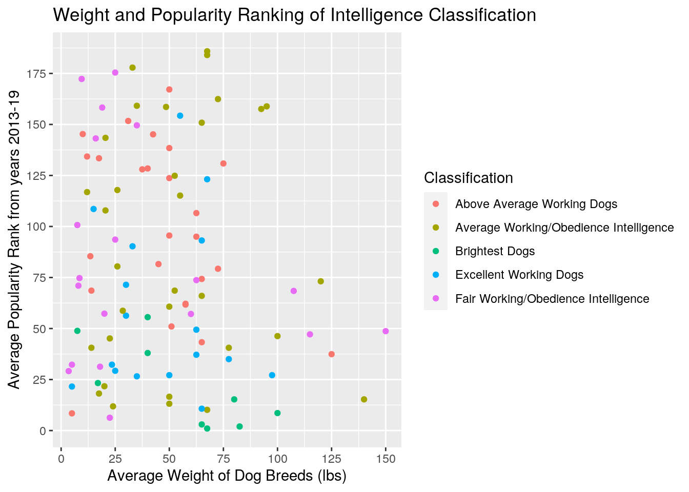 This graph shows a plot between average weight of dog breeds, average height of average popularity ranking, and 5 intelligence classification for all dog breeds. There is not much of a correlation in trends but you can see that above average working dogs tend to skew to a higher popularity ranking (meaning it is lower on a list of 1-193), as it's weight tends to be lower in lbs. You can't really see a relationship between weight and ranking. I changed the scaling on both the y and x axis and had all of them colored by classification.
ggplot(DognoNA, aes(x = Classification, y = AvgRank, fill = Classification)) +
geom_bar(stat = "summary", fun = mean) + scale_fill_brewer(palette = "Pastel2") +
scale_x_discrete(labels = c("Above Avg Wk", "Avg Wk/Ob",
"Brightest", "Excellent", "Fair Wk/Ob")) + labs(x = "Intelligence Classification of Dogs",
y = "Average Popularity Rank through 2013-19", title = "Average Popularity Ranking of Each Dog Intelligence Classification") +
scale_y_continuous(breaks = seq(0, 110, 10)) + geom_errorbar(stat = "summary",
width = 0.5) + theme(legend.text = element_text(size = 6))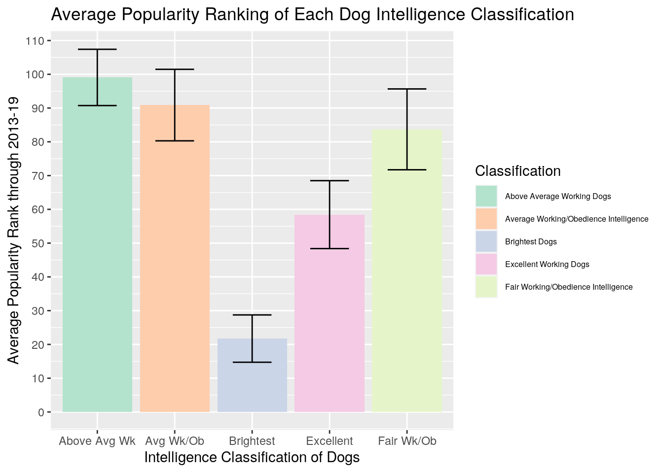 This graphbar shows the number of average rankings per each dog intelligence classifications with a standard error bar. Just looking at the graph you can see that the brightest dogs have a overall smaller average ranking for popularity ranking meaning that it typically tends to be the most popular breeds that fall into this category and people tend to choose/own they dogs. The overall highest average ranking for popularity meaning it tends to be less popular dog breed are the above average working dogs, and people tend to choose/own these dogs less.I changed both x and y scales to make everything neater and more readable. I added color to each classification and changed the font size for the legend. I also changed the sizing of the SE bars.
library(tidyverse)
dgi <- Dogpop %>% full_join(Dogin, by = c(Breed = "Breed"))
dggg <- dgi %>% full_join(Dogbdinfo, by = c(Breed = "Breed"))
dg <- dggg %>% select_if(is.numeric) %>% na.omit()
dg %>% select_if(is.numeric) %>% cor(use = "pair")
## Rank avgReps avght avgwt
## Rank 1.000000000 0.07110275 -0.007939942 -0.11564849
## avgReps 0.071102750 1.00000000 -0.157220883 -0.01488321
## avght -0.007939942 -0.15722088 1.000000000 0.70747102
## avgwt -0.115648490 -0.01488321 0.707471015 1.00000000cormat <- dg %>% select_if(is.numeric) %>% cor(use = "pair")
cordat <- cormat %>% as.data.frame %>% rownames_to_column("var1") %>%
pivot_longer(-1, names_to = "var2", values_to = "corelation")
cordat %>% ggplot(aes(var1, var2, fill = corelation)) + geom_tile() +
geom_text(aes(label = round(corelation, 2))) + xlab("") +
ylab("") + coord_fixed() + scale_fill_gradient2(low = "white",
mid = "pink", high = "red") + theme(axis.text.x = element_text(angle = 90,
vjust = 0.5, hjust = 1))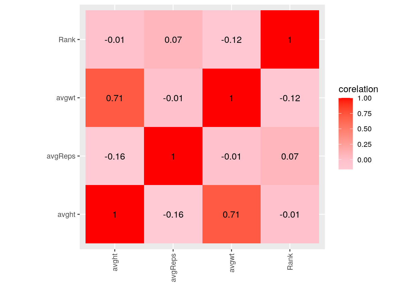 This heat map shows the correlation between 4 numeric variables in the 'dg' dataset. The dg dataset was using the untidyed popularity ranking per year as it made it easier to see the correlations than having it's average so I full joined that with the other tidied datasets and I will be using this one for dimensionality reduction as well. You can see that average height and weight do have a positve correlation meaning that they do affect each other in dog breeds, which is to be expected (taller dog/more it weighs and vice versa), there is a negative correlation between dog intelligence (avgReps) and height and weight (so they don't affect/correlate each other), there is also a negative correlation for height and weights between ranking (so no correlation for ranking and weight or ranking and height), and finally there is a small postive correlation for average reps (Dog intelligence) and ranking (so dog intelligence does affect popularity ranking).
Dimensionality Reduction
library(cluster)
wss <- vector()
for (i in 1:4) {
    dgt <- dg %>% dplyr::select(Rank, avgReps, avght, avgwt) %>%
        kmeans(., i)
    wss[i] <- dgt$tot.withinss
}
ggplot() + geom_point(aes(x = 1:4, y = wss)) + geom_path(aes(x = 1:4,
    y = wss)) + xlab("clusters") + scale_x_continuous(breaks = 1:4)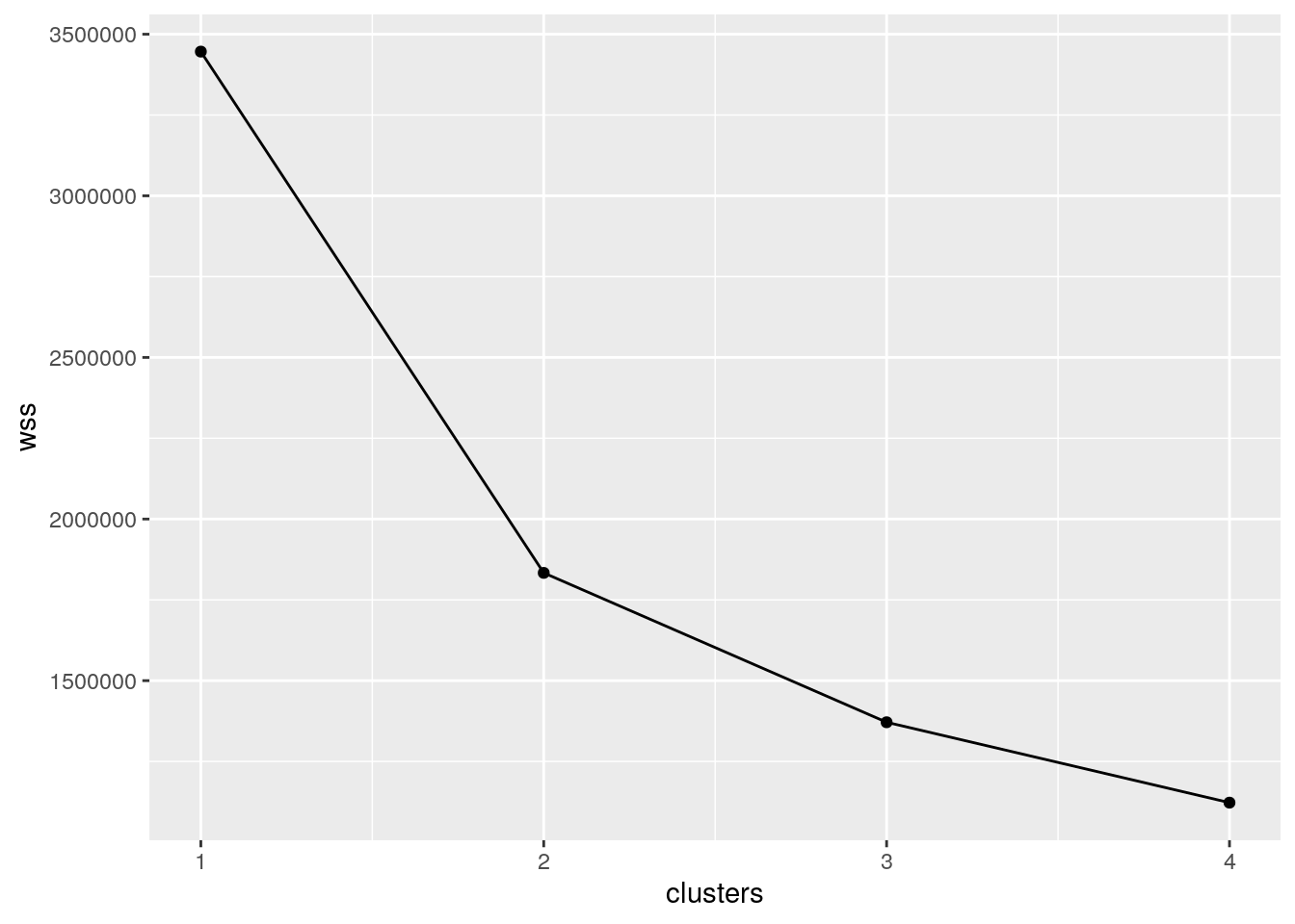
kmeans1 <- dg %>% scale %>% kmeans(2)
kclust <- dg %>% mutate(cluster = as.factor(kmeans1$cluster))
kclust %>% ggplot(aes(avght, avgwt, color = cluster)) + geom_point()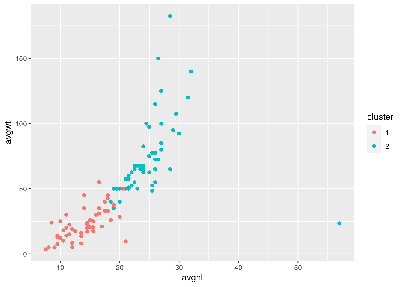
kclust %>% mutate(reps = dg$avgReps) %>% ggplot(aes(avgwt, avght,
color = avgReps, shape = cluster)) + geom_point(size = 3) +
ggtitle("Cluster using kmeans")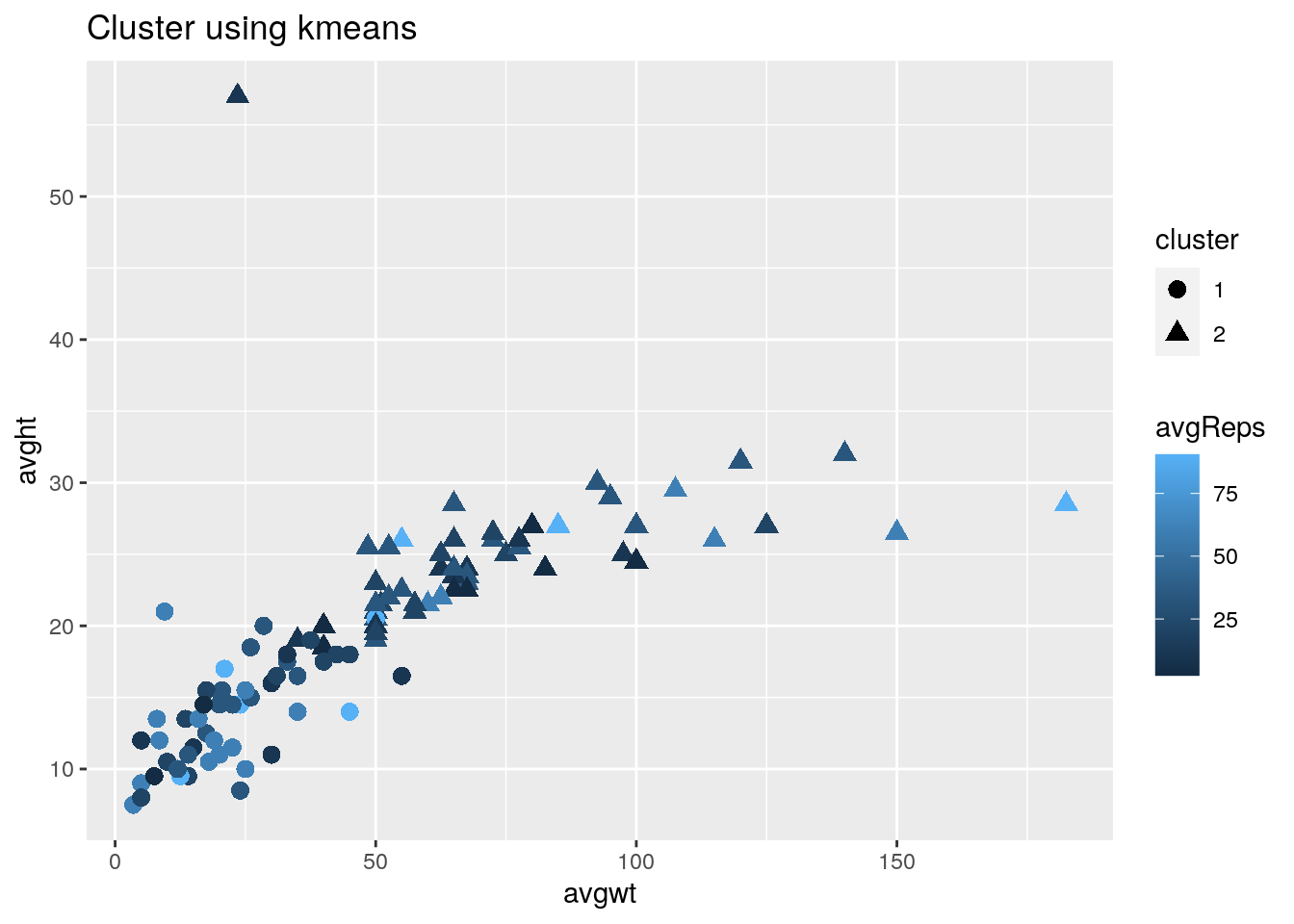 So I first determined the number of clustered I need, and I determined I needed 2 based off the number of numeric variables I had. I used kmeans to cluster my data and create my graphs It's hard to tell but you can see that the lower reps () tend to be spread out between 0-100 average weight and be less than 35 inches of height. You can't really see any other correlations as it is all over the place so associations are hard to see.