November 25, 2020
Modeling
Alejandra Plazola and Map5667
Introduction
This is the 'College' dataset, in which it is a dataset that containing information abbout college majors across the U.S and their median incomes. This dataset is from the American Community Survey 2010-2012 Public Use Microdata Series https://github.com/rfordatascience/tidytuesday/tree/master/data/2018/2018-10-16 https://github.com/rfordatascience/tidytuesday. It has 21 variables and 172 observations. The variable names it contains that are Rank, Major_code, Major, Major_category, Total, Sample_size, Men, Women, ShareWomen, Employed, Full_time, Part_time, Full_time_year_round, Unemployed, Unemployment_rate, Media, P25th, P75th, College_jobs, Non_college_jobs, and Low_wage_jobs.
library(mvtnorm)
library(ggplot2)
library(dplyr)
library(tidyverse)
library(lmtest)
library(glmnet)
College <- readr::read_csv("https://raw.githubusercontent.com/rfordatascience/tidytuesday/master/data/2018/2018-10-16/recent-grads.csv")
cg <- College %>% na.omit()
College %>% group_by(Major_category) %>% count()
## # A tibble: 16 x 2
## # Groups: Major_category [16]
## Major_category n
## <chr> <int>
## 1 Agriculture & Natural Resources 10
## 2 Arts 8
## 3 Biology & Life Science 14
## 4 Business 13
## 5 Communications & Journalism 4
## 6 Computers & Mathematics 11
## 7 Education 16
## 8 Engineering 29
## 9 Health 12
## 10 Humanities & Liberal Arts 15
## 11 Industrial Arts & Consumer Services 7
## 12 Interdisciplinary 1
## 13 Law & Public Policy 5
## 14 Physical Sciences 10
## 15 Psychology & Social Work 9
## 16 Social Science 9# Subsetting data to only have 5 observations for
# Major_Category
College <- College %>% filter(Major_category != "Arts" & Major_category !=
"Interdisciplinary" & Major_category != "Law & Public Policy" &
Major_category != "Industrial Arts & Consumer Services" &
Major_category != "Communications & Journalism" & Major_category !=
"Social Science" & Major_category != "Psychology & Social Work" &
Major_category != "Biology & Life Science" & Major_category !=
"Agriculture & Natural Resources" & Major_category != "Health" &
Major_category != "Physical Sciences")MANOVA
ggplot(College, aes(x = Employed, y = Median)) + geom_point(alpha = 0.1) +
    geom_density_2d(h = 2) + coord_fixed() + facet_wrap(~Major_category)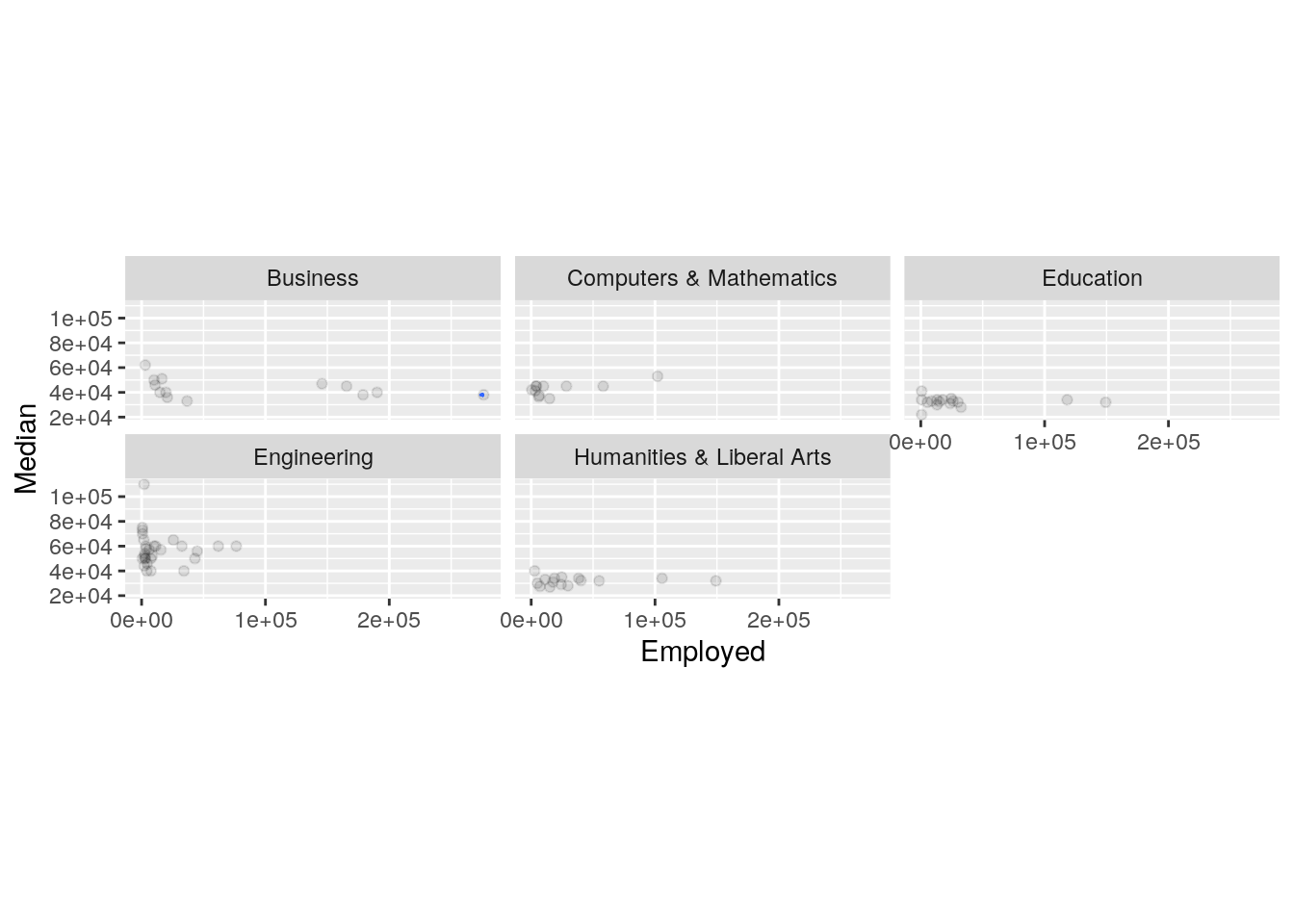
MANC <- manova(cbind(Employed, Median) ~ Major_category, data = College)
summary(MANC)
## Df Pillai approx F num Df den Df Pr(>F)
## Major_category 4 0.77805 12.575 8 158 6.901e-14 ***
## Residuals 79
## ---
## Signif. codes: 0 '***' 0.001 '**' 0.01 '*' 0.05 '.' 0.1 ' ' 1summary.aov(MANC)## Response Employed :
## Df Sum Sq Mean Sq F value Pr(>F)
## Major_category 4 4.5140e+10 1.1285e+10 5.0807 0.001074 **
## Residuals 79 1.7547e+11 2.2211e+09
## ---
## Signif. codes: 0 '***' 0.001 '**' 0.01 '*' 0.05 '.' 0.1 ' ' 1
##
## Response Median :
## Df Sum Sq Mean Sq F value Pr(>F)
## Major_category 4 9576798960 2394199740 28.774 9.28e-15 ***
## Residuals 79 6573456755 83208313
## ---
## Signif. codes: 0 '***' 0.001 '**' 0.01 '*' 0.05 '.' 0.1 ' ' 1College %>% group_by(Major_category) %>% summarize(mean(Employed),
mean(Median))## # A tibble: 5 x 3
## Major_category `mean(Employed)` `mean(Median)`
## <chr> <dbl> <dbl>
## 1 Business 83749. 43538.
## 2 Computers & Mathematics 21627. 42745.
## 3 Education 29990. 32350
## 4 Engineering 14496. 57383.
## 5 Humanities & Liberal Arts 36275. 31913.pairwise.t.test(College$Employed, College$Major_category, p.adj = "none")##
## Pairwise comparisons using t tests with pooled SD
##
## data: College$Employed and College$Major_category
##
## Business Computers & Mathematics Education
## Computers & Mathematics 0.0019 - -
## Education 0.0031 0.6517 -
## Engineering 3.3e-05 0.6703 0.2943
## Humanities & Liberal Arts 0.0095 0.4360 0.7116
## Engineering
## Computers & Mathematics -
## Education -
## Engineering -
## Humanities & Liberal Arts 0.1502
##
## P value adjustment method: nonepairwise.t.test(College$Median, College$Major_category, p.adj = "none")##
## Pairwise comparisons using t tests with pooled SD
##
## data: College$Median and College$Major_category
##
## Business Computers & Mathematics Education
## Computers & Mathematics 0.8325 - -
## Education 0.0015 0.0047 -
## Engineering 1.9e-05 2.1e-05 2.3e-13
## Humanities & Liberal Arts 0.0012 0.0037 0.8944
## Engineering
## Computers & Mathematics -
## Education -
## Engineering -
## Humanities & Liberal Arts 2.6e-13
##
## P value adjustment method: none# Probability of at least one type I error
1 - (0.95^23)## [1] 0.6926431# Bonferroni Correction
0.05/23## [1] 0.002173913A one-way MANOVA was conducted to determine the effect of the Major_Category type (Engineering, Business, Computers&Mathematics, Education, and Humanities&Arts) on two dependent variables (Median and Employed). Based on the MANOVA, there was a significiant difference found between the 5 major categories, Pillai trace=0.77805,pseudo F (4, 158) = 12.575, p < 0.0001. Univariate ANOVAs for each dependent variable were conducted as follow-up tests to the MANOVA, using the Bonferroni method for controlling Type I error rates for multiple comparisons.The univariate ANOVAs for Employed and Media were also significant, F (4, 79) = 5.0807, p < .005, and F (2, 79) = 28.774, p < .0001, respectively.Post hoc analysis was performed conducting pairwise comparisons to determine which Major_Category differed in Employed and Median. All major categories differ based on both Employment and Median income.
There are several assumptions including multivariate normality, equal covariance between two dependent variables, linear relationships among variables, no extreme univariate or multivariate outliers, and no multicollinearity. It is likely that not all assumptions are met based on the density plot for each group as I can see some outliers for some.
I performed 1 MANOVA, 2 ANOVAS, and 20 t tests so the bonferroni significance level is α = .05/20 = .002173913. The probability of at least one type I error, unadjusted, is 0.6926431. All three Species were found to differ significantly from each other in terms of sepal length and petal width after adjusting for multiple comparisons (bonferroni α = .05/9 = .0056). Both Median and Employed are still significant after finding bonferroni corrected significance level.
Randomization Test
set.seed(348)
summary(aov(Median ~ Major_category, data = College))
## Df Sum Sq Mean Sq F value Pr(>F)
## Major_category 4 9.577e+09 2.394e+09 28.77 9.28e-15 ***
## Residuals 79 6.573e+09 8.321e+07
## ---
## Signif. codes: 0 '***' 0.001 '**' 0.01 '*' 0.05 '.' 0.1 ' ' 1obs_F <- 28.77 #this is the observed F-statistic
Fs <- replicate(5000, {
# do everything in curly braces 5000 times and save the
# output
new <- College %>% mutate(Med = sample(Median)) #randomly permute response variable
# compute the F-statistic by hand
SSW <- new %>% group_by(Major_category) %>% summarize(SSW = sum((Med -
mean(Med))^2)) %>% summarize(sum(SSW)) %>% pull
SSB <- new %>% mutate(mean = mean(Med)) %>% group_by(Major_category) %>%
mutate(groupmean = mean(Med)) %>% summarize(SSB = sum((mean -
groupmean)^2)) %>% summarize(sum(SSB)) %>% pull
(SSB/2)/(SSW/57) #compute F statistic (num df = K-1 = 3-1, denom df = N-K = 60-3)
})
hist(Fs, prob = T)
abline(v = obs_F, col = "red", add = T)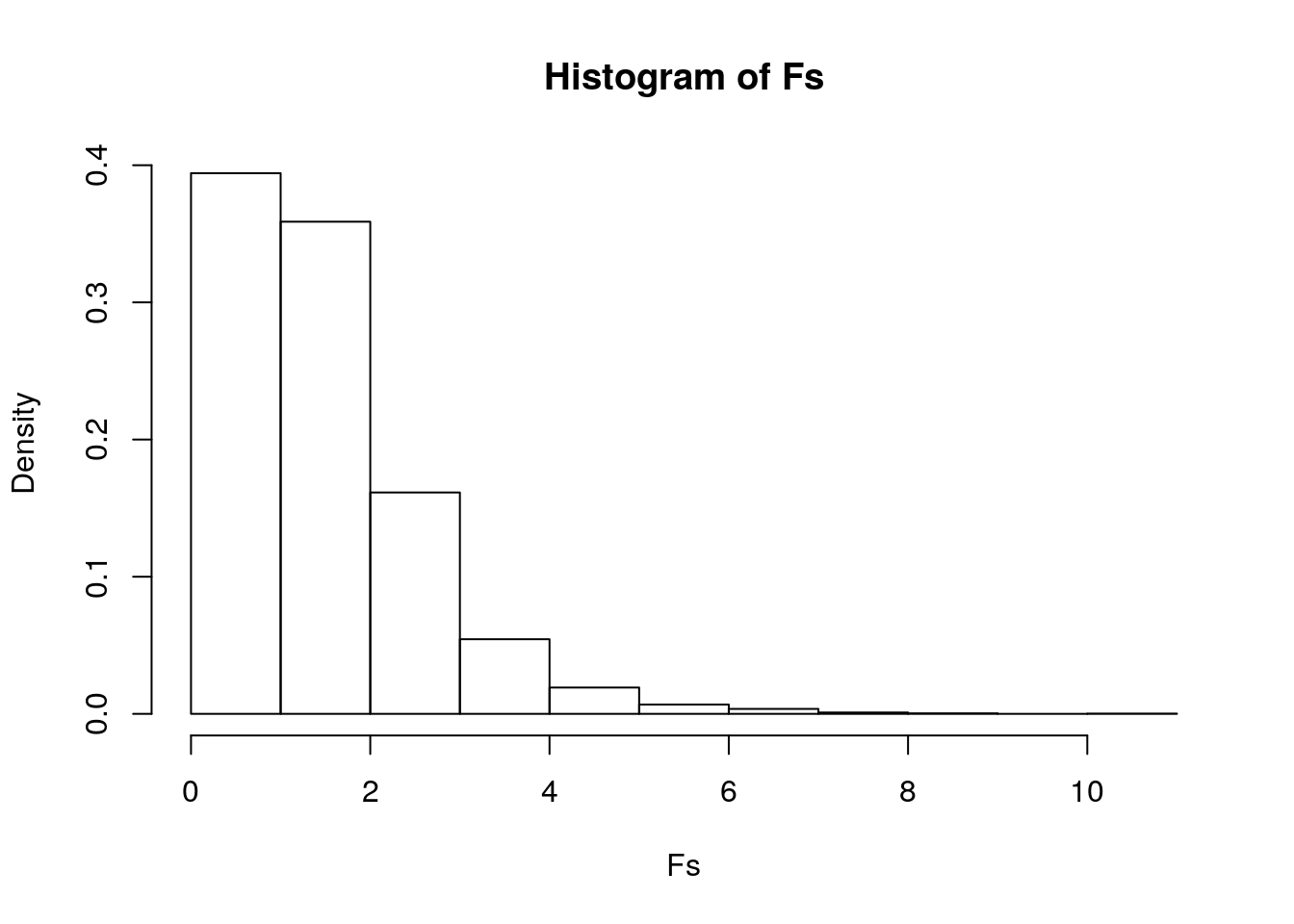
mean(Fs > obs_F)## [1] 0The null hypothesis is that the true mean of Median income is the same for all 5 major category groups(Engineering, Computers&Mathematics,Education, Humanities&Arts, and Business). The alternative hypothesis is that at least of the means of Median incaome for all 5 major category groups differ. I conducted an ANOVA/Fstat test and the p-value for mean(Fs>obs_F) is 0. This means none of our 5000 F stats generated under the null hypothesis were bigger than our actual F stat of 28.77 and means that it definitely rejected the null hypothesis and that major category groups do differ.
Linear Regression Model
College$M <- College$Men - mean(College$Men)

College$W <- College$Women - mean(College$Women)

fit1 <- lm(Median ~ W + M, data = College)
summary(fit1)
##
## Call:
## lm(formula = Median ~ W + M, data = College)
##
## Residuals:
## Min 1Q Median 3Q Max
## -23071 -9453 -2661 6324 64526
##
## Coefficients:
## Estimate Std. Error t value Pr(>|t|)
## (Intercept) 4.401e+04 1.435e+03 30.661 < 2e-16 ***
## W -1.933e-01 5.506e-02 -3.511 0.000733 ***
## M 1.414e-01 6.048e-02 2.339 0.021822 *
## ---
## Signif. codes: 0 '***' 0.001 '**' 0.01 '*' 0.05 '.' 0.1 ' ' 1
##
## Residual standard error: 13150 on 81 degrees of freedom
## Multiple R-squared: 0.1321, Adjusted R-squared: 0.1107
## F-statistic: 6.165 on 2 and 81 DF, p-value: 0.00322ggplot(College, aes(y = M, x = W, color = Median)) + geom_point() +
geom_smooth(method = "lm", se = FALSE)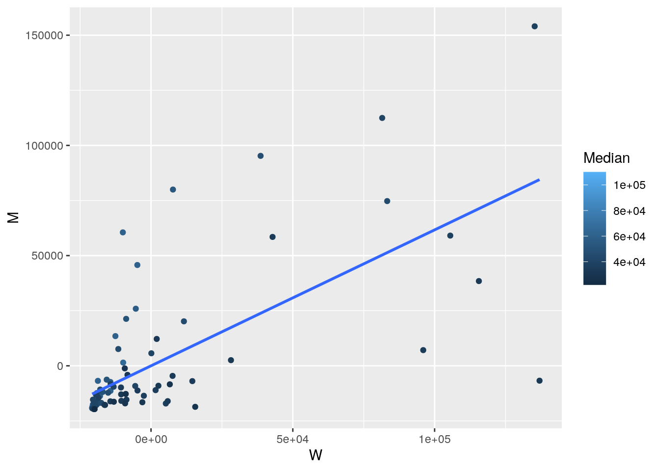
qqnorm(College$M)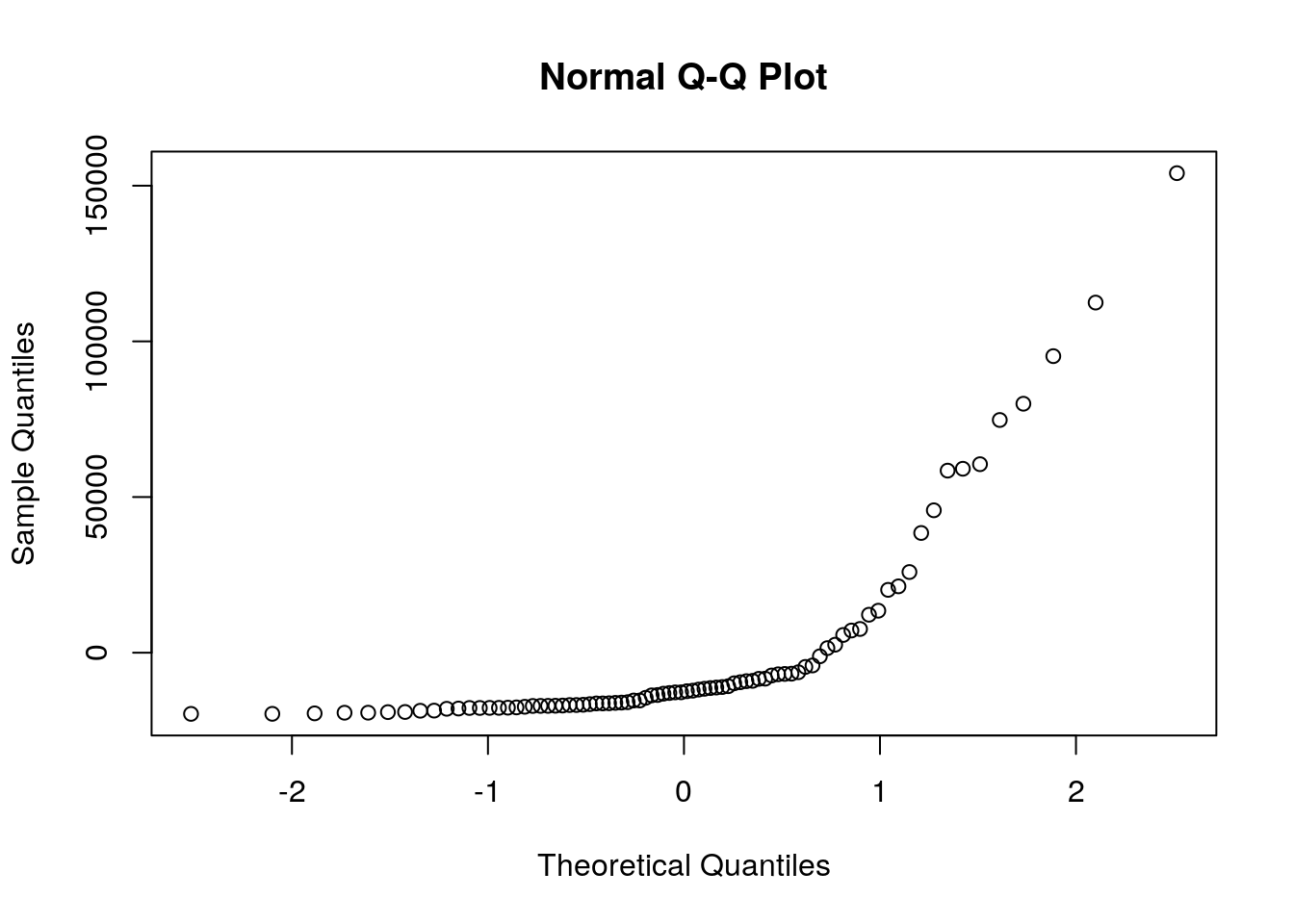
qqnorm(College$W)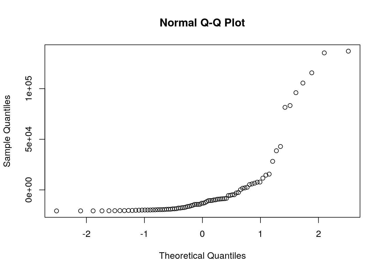
shapiro.test(head(College$M))##
## Shapiro-Wilk normality test
##
## data: head(College$M)
## W = 0.56745, p-value = 0.000182shapiro.test(head(College$W))##
## Shapiro-Wilk normality test
##
## data: head(College$W)
## W = 0.51881, p-value = 4.234e-05bptest(fit1)##
## studentized Breusch-Pagan test
##
## data: fit1
## BP = 1.7016, df = 2, p-value = 0.4271library(sandwich)
coeftest(fit1, vcov = vcovHC(fit1))##
## t test of coefficients:
##
## Estimate Std. Error t value Pr(>|t|)
## (Intercept) 44007.14286 1453.53766 30.2759 < 2.2e-16 ***
## W -0.19331 0.06623 -2.9188 0.004548 **
## M 0.14143 0.05465 2.5880 0.011439 *
## ---
## Signif. codes: 0 '***' 0.001 '**' 0.01 '*' 0.05 '.' 0.1 ' ' 1summary(fit1)$r.sq## [1] 0.1321102fit2 <- lm(Median ~ Men, data = College) #main effects of lat
summary(fit2)##
## Call:
## lm(formula = Median ~ Men, data = College)
##
## Residuals:
## Min 1Q Median 3Q Max
## -22054 -10295 -3865 7221 65950
##
## Coefficients:
## Estimate Std. Error t value Pr(>|t|)
## (Intercept) 4.405e+04 1.796e+03 24.529 <2e-16 ***
## Men -2.400e-03 4.746e-02 -0.051 0.96
## ---
## Signif. codes: 0 '***' 0.001 '**' 0.01 '*' 0.05 '.' 0.1 ' ' 1
##
## Residual standard error: 14030 on 82 degrees of freedom
## Multiple R-squared: 3.118e-05, Adjusted R-squared: -0.01216
## F-statistic: 0.002557 on 1 and 82 DF, p-value: 0.9598fit3 <- lm(Median ~ Women, data = College)
summary(fit3)##
## Call:
## lm(formula = Median ~ Women, data = College)
##
## Residuals:
## Min 1Q Median 3Q Max
## -24115 -10415 -950 7291 63812
##
## Coefficients:
## Estimate Std. Error t value Pr(>|t|)
## (Intercept) 4.622e+04 1.710e+03 27.031 <2e-16 ***
## Women -1.061e-01 4.159e-02 -2.551 0.0126 *
## ---
## Signif. codes: 0 '***' 0.001 '**' 0.01 '*' 0.05 '.' 0.1 ' ' 1
##
## Residual standard error: 13510 on 82 degrees of freedom
## Multiple R-squared: 0.07351, Adjusted R-squared: 0.06221
## F-statistic: 6.506 on 1 and 82 DF, p-value: 0.01261# install.packages('interactions')
library(interactions)
interact_plot(fit1, M, W) #interaction plot 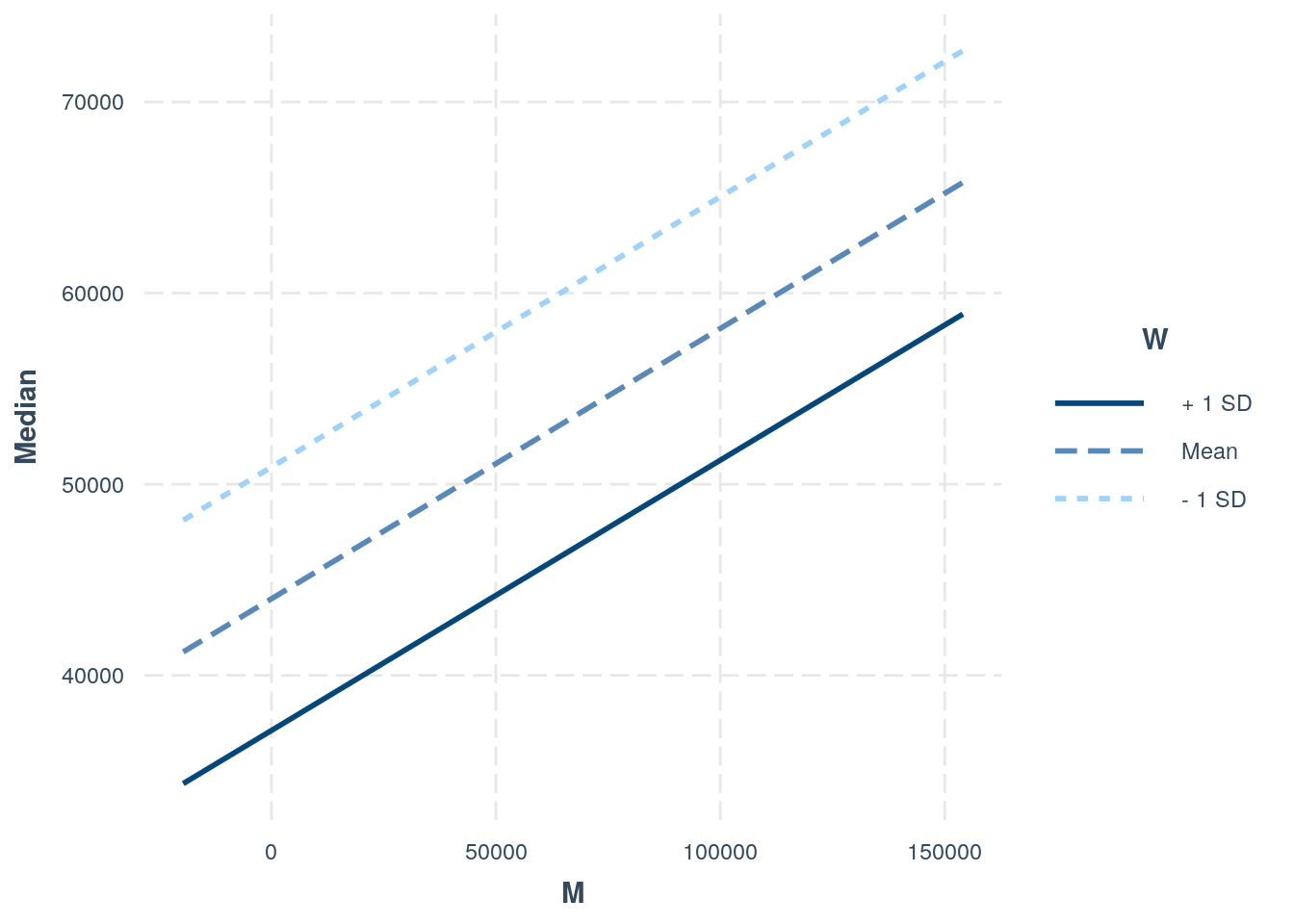 For every one unit increase in Median income, the total number of Women decreases by .01933 units and the total number of Men increases by .01414 units. The linearity assumption is violated based on the ggplot. There does not seem to be normality based on the q-q plots. From the Shapiro-Wilk, the p-value < 0.05 implying that the distribution of the data are significantly different from normal distribution; meaning we cannot assume normalitiy. Based on the Breusch-Pagan test, the p-Value > 0.05 indicates that the null hypothesis can rejected and therefore heterscedasticity does exists. With the robust standard errors, the t-values increases for the intercept and M, the t-values for W decreases, the p-values for Intercept and M decreased, and the p-values for W increased. The proportion of the variation in the outcome explained by this model is 0.1321102.
Bootstrapped Standard Error
set.seed(348)
fit4 <- lm(Median ~ Men * Women, data = College)
boot_sd <- College[sample(nrow(College), replace = T), ]
samp_distn <- replicate(1000, {
    boot_sd <- College[sample(nrow(College), replace = T), ]
    fit5 <- lm(Median ~ Men * Women, data = boot_sd)
    coef(fit5)
})
samp_distn %>% t %>% as.data.frame %>% summarize_all(sd)
## (Intercept) Men Women Men:Women
## 1 2436.675 0.07474423 0.1286051 1.675863e-06# Uncorrected SEs
summary(fit4)##
## Call:
## lm(formula = Median ~ Men * Women, data = College)
##
## Residuals:
## Min 1Q Median 3Q Max
## -23170 -9449 -2706 6294 64437
##
## Coefficients:
## Estimate Std. Error t value Pr(>|t|)
## (Intercept) 4.534e+04 1.949e+03 23.265 < 2e-16 ***
## Men 1.342e-01 8.733e-02 1.537 0.12831
## Women -1.973e-01 6.541e-02 -3.017 0.00343 **
## Men:Women 1.032e-07 8.944e-07 0.115 0.90839
## ---
## Signif. codes: 0 '***' 0.001 '**' 0.01 '*' 0.05 '.' 0.1 ' ' 1
##
## Residual standard error: 13240 on 80 degrees of freedom
## Multiple R-squared: 0.1323, Adjusted R-squared: 0.09971
## F-statistic: 4.064 on 3 and 80 DF, p-value: 0.009666# Corrected SEs
coeftest(fit4, vcov = vcovHC(fit4))##
## t test of coefficients:
##
## Estimate Std. Error t value Pr(>|t|)
## (Intercept) 4.5342e+04 2.2933e+03 19.7712 < 2e-16 ***
## Men 1.3420e-01 6.1517e-02 2.1815 0.03208 *
## Women -1.9733e-01 9.8574e-02 -2.0018 0.04870 *
## Men:Women 1.0325e-07 8.4765e-07 0.1218 0.90336
## ---
## Signif. codes: 0 '***' 0.001 '**' 0.01 '*' 0.05 '.' 0.1 ' ' 1The SEs for the uncorrected SEs for the Intercept and Women seem to be smaller than the corrected SEs. The SEs for the uncorrected SEs for Men and Men:Women tend to be bigger than corrected SEs. The p-values for the uncorrected SEs for intercept, Men, Men:Women seem to be lower than the p-values for the corrected SEs. The p-value for Women for the uncorrected SEs seem to be higher than the p-value for the corrected SE.
Logistic Regression Model
College_new <- College %>% mutate(Major_cat = if_else(Major_category ==
    "Engineering", "Eng", "Other"))
College_new$y <- ifelse(College_new$Major_cat == "Eng", 1, 0)
fit6 <- glm(y ~ P25th + P75th, data = College_new, family = "binomial")
coeftest(fit6)
##
## z test of coefficients:
##
## Estimate Std. Error z value Pr(>|z|)
## (Intercept) -1.0572e+01 2.2396e+00 -4.7205 2.353e-06 ***
## P25th 1.1565e-04 6.2369e-05 1.8543 0.063703 .
## P75th 1.0598e-04 3.9637e-05 2.6737 0.007502 **
## ---
## Signif. codes: 0 '***' 0.001 '**' 0.01 '*' 0.05 '.' 0.1 ' ' 1exp(coef(fit6))## (Intercept) P25th P75th
## 2.561903e-05 1.000116e+00 1.000106e+00College_new$probs <- predict(fit6, type = "response")
table(predict = as.numeric(College_new$probs > 0.5), truth = College_new$y) %>%
addmargins()## truth
## predict 0 1 Sum
## 0 48 5 53
## 1 7 24 31
## Sum 55 29 84# Sensitivity(TPR)
24/29## [1] 0.8275862# Specificity(TNR)
48/55## [1] 0.8727273# Precision(PPV)
24/31## [1] 0.7741935## GIVE IT PREDICTED PROBS AND TRUTH LABELS (0/1), RETURNS
## VARIOUS DIAGNOSTICS
class_diag <- function(probs, truth) {
# CONFUSION MATRIX: CALCULATE ACCURACY, TPR, TNR, PPV
if (is.character(truth) == TRUE)
truth <- as.factor(truth)
if (is.numeric(truth) == FALSE & is.logical(truth) == FALSE)
truth <- as.numeric(truth) - 1
tab <- table(factor(probs > 0.5, levels = c("FALSE", "TRUE")),
factor(truth, levels = c(0, 1)))
acc = sum(diag(tab))/sum(tab)
sens = tab[2, 2]/colSums(tab)[2]
spec = tab[1, 1]/colSums(tab)[1]
ppv = tab[2, 2]/rowSums(tab)[2]
f1 = 2 * (sens * ppv)/(sens + ppv)
# CALCULATE EXACT AUC
ord <- order(probs, decreasing = TRUE)
probs <- probs[ord]
truth <- truth[ord]
TPR = cumsum(truth)/max(1, sum(truth))
FPR = cumsum(!truth)/max(1, sum(!truth))
dup <- c(probs[-1] >= probs[-length(probs)], FALSE)
TPR <- c(0, TPR[!dup], 1)
FPR <- c(0, FPR[!dup], 1)
n <- length(TPR)
auc <- sum(((TPR[-1] + TPR[-n])/2) * (FPR[-1] - FPR[-n]))
data.frame(acc, sens, spec, ppv, f1, auc)
}
probs1 <- predict(fit6, type = "response")
class_diag(probs1, College_new$y)## acc sens spec ppv f1 auc
## 1 0.8571429 0.8275862 0.8727273 0.7741935 0.8 0.9213166College_new$logit <- predict(fit6, type = "link")
College_new %>% ggplot() + geom_density(aes(logit, color = Major_cat,
fill = Major_cat), alpha = 0.4) + theme(legend.position = c(0.83,
0.83)) + geom_vline(xintercept = 0) + xlab("logit (log-odds)") +
geom_rug(aes(logit, color = Major_cat))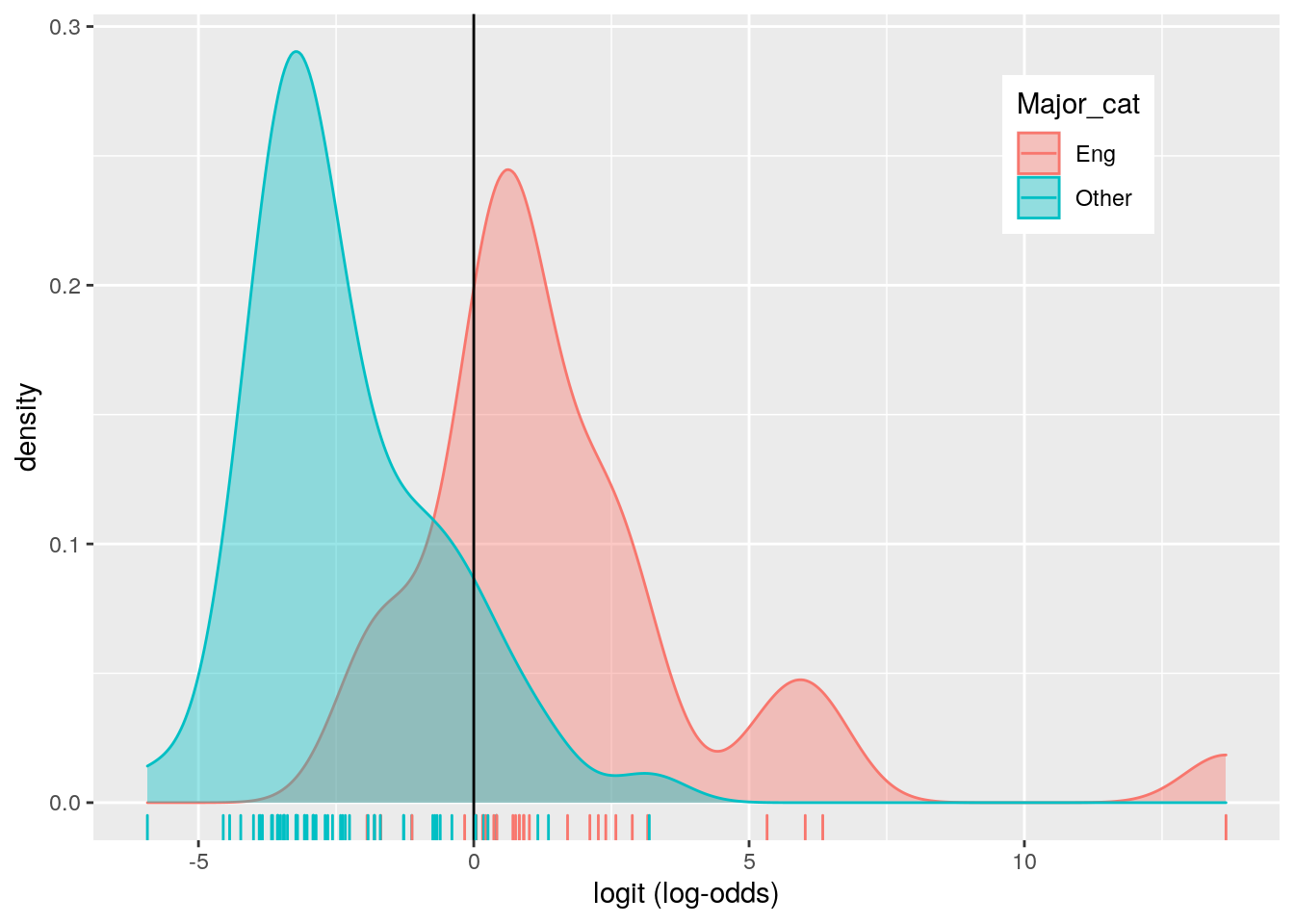
library(plotROC)
# ROCCurve
ROCplot <- ggplot(College_new) + geom_roc(aes(d = y, m = probs),
    n.cuts = 0) + geom_segment(aes(x = 0, xend = 1, y = 0, yend = 1),
    lty = 2)
ROCplot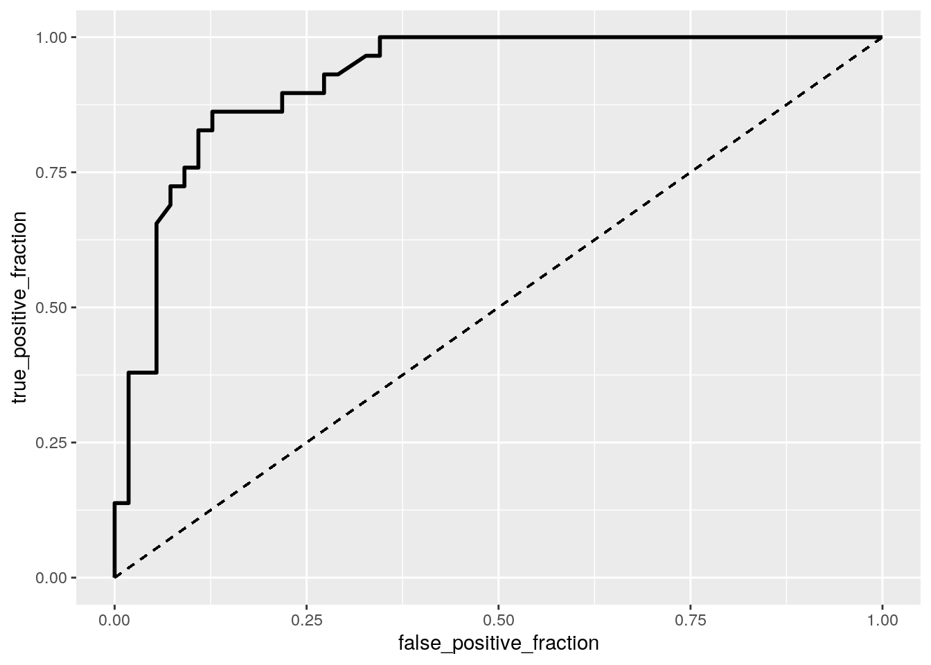
# AUC
calc_auc(ROCplot)
## PANEL group AUC
## 1 1 -1 0.9213166The logistic regression model tells us the odds of being an Engineering major for when p25th income=0 and p75th income=0 is 2.561903e-05. Controlling for Engineering Major and P75th income, for every additional unit of P25th the odds of it being an Engineering major it increases by 1.000116. Controlling for Engineering and P25th income, the odds of it an Engineering major to increase income is by 1.000106.
The TPR/Sensitivity is 0.8275862, and the TNR/Specificity is 0.8727273: this means the model is good at predictings that the probability a major being either Engineering or other(the other 4 grouped together).The PPV/Precision is .7741935 which gives us the proportion of those majors classified as Engineering being Engineering. The accurarcy is .8571429 meaning it seems to be pretty good. The AUC found is 0.9213166, meaning the this model is "great!" at predicting between postive and negative classes.
The ROC curves shows the trade-off between TPR and TNR. The AUC caclculated is 0.9213166, meaning the this model is "great!", there is no change (this an error on my part).
Logistic regression Binary
# log regression using binary
cn <- College_new %>% select(-c("Major", "Major_category", "Major_cat"))
fit8 <- glm(y ~ ., data = cn, family = "binomial")
coeftest(fit8)
##
## z test of coefficients:
##
## Estimate Std. Error z value Pr(>|z|)
## (Intercept) 5.5485e+15 8.8044e+07 63019497 < 2.2e-16 ***
## Rank -1.8253e+13 3.8359e+05 -47584893 < 2.2e-16 ***
## Major_code -7.1379e+11 6.0623e+03 -117743093 < 2.2e-16 ***
## Total 2.3652e+11 8.7626e+03 26992064 < 2.2e-16 ***
## Men -1.1283e+11 1.5267e+03 -73903241 < 2.2e-16 ***
## Women NA NA NA NA
## ShareWomen -4.2508e+15 6.6713e+07 -63717250 < 2.2e-16 ***
## Sample_size -1.5769e+12 1.8438e+05 -8552133 < 2.2e-16 ***
## Employed -1.7954e+12 2.0057e+04 -89513548 < 2.2e-16 ***
## Full_time 1.3103e+12 1.7577e+04 74549230 < 2.2e-16 ***
## Part_time 1.1620e+12 1.5114e+04 76883612 < 2.2e-16 ***
## Full_time_year_round 3.6174e+11 1.0886e+04 33230886 < 2.2e-16 ***
## Unemployed -8.6835e+11 2.6140e+04 -33219897 < 2.2e-16 ***
## Unemployment_rate -5.5195e+15 2.8385e+08 -19444982 < 2.2e-16 ***
## Median -2.1246e+10 2.7160e+03 -7822417 < 2.2e-16 ***
## P25th 3.4401e+10 2.0545e+03 16744641 < 2.2e-16 ***
## P75th -1.8411e+10 1.5804e+03 -11649499 < 2.2e-16 ***
## College_jobs -1.3887e+10 1.6381e+03 -8477182 < 2.2e-16 ***
## Non_college_jobs 5.9507e+10 3.2233e+03 18461503 < 2.2e-16 ***
## Low_wage_jobs -1.3730e+11 1.0496e+04 -13080908 < 2.2e-16 ***
## [ reached getOption("max.print") -- omitted 4 rows ]
## ---
## Signif. codes: 0 '***' 0.001 '**' 0.01 '*' 0.05 '.' 0.1 ' ' 1exp(coef(fit8))## (Intercept) Rank Major_code
## Inf 0 0
## Total Men Women
## Inf 0 NA
## ShareWomen Sample_size Employed
## 0 0 0
## Full_time Part_time Full_time_year_round
## Inf Inf Inf
## Unemployed Unemployment_rate Median
## 0 0 0
## P25th P75th College_jobs
## Inf 0 0
## Non_college_jobs Low_wage_jobs M
## Inf 0 NA
## W probs logit
## NA Inf NAprobs2 <- predict(fit8, type = "response")
class_diag(probs2, cn$y)## acc sens spec ppv f1 auc
## 1 0.9404762 0.9655172 0.9272727 0.875 0.9180328 0.946395summary(fit8)##
## Call:
## glm(formula = y ~ ., family = "binomial", data = cn)
##
## Deviance Residuals:
## Min 1Q Median 3Q Max
## -8.49 0.00 0.00 0.00 8.49
##
## Coefficients: (4 not defined because of singularities)
## Estimate Std. Error z value Pr(>|z|)
## (Intercept) 5.548e+15 8.804e+07 63019497 <2e-16 ***
## Rank -1.825e+13 3.836e+05 -47584893 <2e-16 ***
## Major_code -7.138e+11 6.062e+03 -117743093 <2e-16 ***
## Total 2.365e+11 8.763e+03 26992064 <2e-16 ***
## Men -1.128e+11 1.527e+03 -73903241 <2e-16 ***
## Women NA NA NA NA
## ShareWomen -4.251e+15 6.671e+07 -63717250 <2e-16 ***
## Sample_size -1.577e+12 1.844e+05 -8552133 <2e-16 ***
## Employed -1.795e+12 2.006e+04 -89513548 <2e-16 ***
## Full_time 1.310e+12 1.758e+04 74549230 <2e-16 ***
## Part_time 1.162e+12 1.511e+04 76883612 <2e-16 ***
## Full_time_year_round 3.617e+11 1.089e+04 33230886 <2e-16 ***
## Unemployed -8.684e+11 2.614e+04 -33219897 <2e-16 ***
## Unemployment_rate -5.520e+15 2.839e+08 -19444982 <2e-16 ***
## Median -2.125e+10 2.716e+03 -7822417 <2e-16 ***
## P25th 3.440e+10 2.054e+03 16744641 <2e-16 ***
## P75th -1.841e+10 1.580e+03 -11649499 <2e-16 ***
## College_jobs -1.389e+10 1.638e+03 -8477182 <2e-16 ***
## Non_college_jobs 5.951e+10 3.223e+03 18461503 <2e-16 ***
## Low_wage_jobs -1.373e+11 1.050e+04 -13080908 <2e-16 ***
## [ reached getOption("max.print") -- omitted 4 rows ]
## ---
## Signif. codes: 0 '***' 0.001 '**' 0.01 '*' 0.05 '.' 0.1 ' ' 1
##
## (Dispersion parameter for binomial family taken to be 1)
##
## Null deviance: 108.27 on 83 degrees of freedom
## Residual deviance: 360.44 on 64 degrees of freedom
## AIC: 400.44
##
## Number of Fisher Scoring iterations: 12set.seed(348)
k = 10
data <- cn[sample(nrow(cn)), ]
folds <- cut(seq(1:nrow(cn)), breaks = k, labels = F)
diags <- NULL
for (i in 1:k) {
train <- data[folds != i, ]
test <- data[folds == i, ]
truth <- test$y
fit <- glm(y ~ ., data = train, family = "binomial")
probs <- predict(fit, newdata = test, type = "response")
diags <- rbind(diags, class_diag(probs, truth))
}
summarize_all(diags, mean)## acc sens spec ppv f1 auc
## 1 0.7638889 0.735 0.7828571 0.6666667 0.6797619 0.8003571# lasso regression
set.seed(348)
cn <- College_new %>% select(-c("Major", "Major_category", "Major_cat"))
library(glmnet)
data(cn)
y <- as.matrix(cn$y)
x <- cn %>% select(-y) %>% mutate_all(scale) %>% as.matrix
head(x)## Rank Major_code Total Men Women ShareWomen
## [1,] -1.334998 -0.5954497 -0.6135406 -0.54597552 -0.5765891 -1.3952364
## [2,] -1.316422 -0.5973626 -0.6389159 -0.58843378 -0.5823396 -1.4736612
## [3,] -1.297847 -0.5980003 -0.6373129 -0.58701645 -0.5808248 -1.2591408
## [4,] -1.279271 -0.5967250 -0.6308689 -0.57475347 -0.5807126 -1.4507725
## Sample_size Employed Full_time Part_time Full_time_year_round
## [1,] -0.5236655 -0.6015220 -0.5834324 -0.6517978 -0.5711890
## [2,] -0.5656982 -0.6274359 -0.6117473 -0.6602564 -0.5940255
## [3,] -0.5714958 -0.6272807 -0.6117035 -0.6633861 -0.5953639
## [4,] -0.5526536 -0.6251471 -0.6005133 -0.6619481 -0.5855489
## Unemployed Unemployment_rate Median P25th P75th College_jobs
## [1,] -0.6129443 -1.6039785 4.730927 5.6640426 4.071532 -0.5993097
## [2,] -0.6006506 1.5782654 2.221831 2.0320334 2.027737 -0.6614842
## [3,] -0.6183228 -1.4199900 2.078454 1.5780323 2.903649 -0.6559179
## [4,] -0.6121759 -0.5821417 1.863388 0.9424307 1.443795 -0.6520845
## Non_college_jobs Low_wage_jobs M W probs logit
## [1,] -0.5185841 -0.5265120 -0.54597552 -0.5765891 1.903466 4.907594
## [2,] -0.5230610 -0.5485560 -0.58843378 -0.5823396 1.889406 2.106488
## [3,] -0.5264501 -0.5562637 -0.58701645 -0.5808248 1.898339 2.446391
## [4,] -0.5295462 -0.5562637 -0.57475347 -0.5807126 1.748794 1.283963
## [ reached getOption("max.print") -- omitted 2 rows ]cv <- cv.glmnet(x, y)
lasso1 <- glmnet(x, y, lambda = cv$lambda.1se)
coef(lasso1)## 24 x 1 sparse Matrix of class "dgCMatrix"
## s0
## (Intercept) 0.34523810
## Rank -0.03610480
## Major_code -0.09511901
## Total .
## Men .
## Women .
## ShareWomen -0.08307175
## Sample_size .
## Employed .
## Full_time .
## Part_time .
## Full_time_year_round .
## Unemployed .
## Unemployment_rate .
## Median 0.05774517
## P25th .
## P75th .
## College_jobs .
## Non_college_jobs .
## Low_wage_jobs .
## M .
## W .
## probs 0.12926262
## logit .prob <- predict(lasso1, newx = x, type = "response")
class_diag(prob, cn$y)## acc sens spec ppv f1 auc
## 1 0.8928571 0.862069 0.9090909 0.8333333 0.8474576 0.9768025k = 10
data <- cn %>% sample_frac #put rows of dataset in random order
folds <- ntile(1:nrow(data), n = 10) #create fold labels
diags <- NULL
for (i in 1:k) {
train <- data[folds != i, ] #create training set (all but fold i)
test <- data[folds == i, ] #create test set (just fold i)
truth <- test$y #save truth labels from fold i
fit <- glm(y ~ Rank + Major_code + ShareWomen + Median, data = train,
family = "binomial")
probs <- predict(fit, newdata = test, type = "response")
diags <- rbind(diags, class_diag(probs, truth))
}
diags %>% summarize_all(mean)## acc sens spec ppv f1 auc
## 1 0.8847222 0.8738095 0.869881 0.8490476 0.8389744 0.9580952The logistic regression using Binary variables acc= .9404762 meaning it is pretty much accurate at predicting, sens= 0.9655172, spec=0.9272727, ppv=0.875, and AUC=0.946395. This model is a great fit for the predicted probilities of Engineering. The 10-fold CV model's acc=0.7638889, sens=0.735 spec=0.7828571, ppv=0.6666667, and AUC=0.8003571. The AUC is fair and when compared to original logistic regression AUC is decreased so the out of sampling isn't good in showing the model.
The variables retained are Rank, Major_code, ShareWomen, and Median. The lasso regression cv performance shows acc=0.8928571, sens=0.862069, spec=0.9090909 and ppv= 0.8333333. The AUC of the lasso regression is 0.9768025, which means it is great and when compared to past AUC it is the highest.
The out-of-sample AUC of the 10-fold CV of the lasso variables selected is 0.9580952. When comparing the AUC to the logistic regression above it is higher but lower than lasso regression cv.